Pandas Pivot Tables: A Comprehensive Guide for Data Science
Python is one of the widely-used programming languages among developers due to its simplicity and larger community support. Python is also becoming a handy language in the Artificial Intelligence (AI) and Machine Learning (ML) sectors as it supports various built-in and external libraries related to those technologies.

One of the popular libraries supported by Python is Pandas, and this library is used when we perform general operations with data sets, such as cleaning, exploring, analyzing, and manipulating data.
In this blog, we will learn one of the major features of Pandas library: Pivot tables and how to create one with examples.
Before going into the Pivot tables, let’s quickly look at the Data pivoting and Pandas pivot() function.
Data pivoting and Pivot () function in Pandas.
Data pivoting is re-arranging the data in our DataFrame so we can easily understand and analyze it as we need.
Note: DataFrame is a data structure where we can store data in a two-dimensional table with columns and rows. It is more like a spreadsheet in Excel.
With data pivoting, we can perform the following tasks.
- Move an object and its related data from a row to a column or column to a row.
- Change the order of objects in the rows or columns.
Python pandas provides a function called pivot() to pivot our data.
Below is the syntax of the pivot() function.
DataFrame.pivot(index=None, columns=None, values=None)
Let’s understand the components of this syntax.
- DataFrame: Here, we include the name of our DataFrame.
- pivot (): This is the function provided by Pandas to pivot our data.
As you can see, inside the pivot() function, three parameters are to be defined.
- index: In this parameter, we will define the column, which will be used to identify and order the rows vertically.
- columns: Here, we will define the column which of its values will be the new columns of the new DataFrame.
- values: This can be a column or columns that will fill our new DataFrame’s cells.
Let’s understand what we have learned so far through an example. Firstly, we can create a DataFrame, as shown below.
import pandas as pd

df = pd.DataFrame({'Restaurant name' : ['ABC', 'ABC', 'PQR', 'PQR', 'PQR', 'XYZ', 'XYZ', 'XYZ'],
                   'Owner' : ['John', 'John', 'Mary', 'Mary', 'Mary', 'Kevin', 'Kevin', 'Kevin'],
                   'Account manager' : ['Linda', 'Linda', 'Roy', 'Roy', 'Roy', 'Linda', 'Linda', 'Linda'],
                   'Food item' : ['Pizza', 'Sandwich', 'Pizza', 'Burger', 'Pasta', 'Sandwich', 'Burger', 'Pasta'],
                   'Sold amount': [20, 45, 10, 30, 5, 35, 25, 15],
                   'Sale price': [4000, 9000, 2000, 1500, 1500, 7000, 1250, 4500]})

print(df)
The above DataFrame has data from three restaurants (ABC, PQR, and XYZ), such as owners (John, Mary, and Kevin), account managers (Linda and Roy), Sold amount, and Sale prices.
When we print the DataFrame (df), we see it below.

Now, assume that we want to filter out and analyze the sales of the food items made by each restaurant. We can use the pivot() function as below.
Sales_amount = df.pivot(index='Restaurant name', columns='Food item', values='Sale price')

print(Sales_amount)
Here, we have set ‘Restaurant name’ as the ‘index.’ Our new DataFrame will have each food item as a new column by choosing ‘Food item’ as the ‘columns’ parameter. Since we need to analyze the sale prices, we set ‘Sale price’ as the ‘values’.
The output is as follows.

As you can see, we can easily use the pivot() function to analyze our DataFrame according to our needs.
But what if we want to find the total sale price or total sold amount of the food items?
We cannot accomplish this task with the pivot() function because it is not designed for aggregation-related operations.
This is where the pivot table comes in to help. Let’s see what a Pivot table is in Pandas.
[blog-subscribe]
What is a Pandas Pivot Table?
The pivot table is similar to the pivot() function but gives us more control over the DataFrame. Simply, it is more powerful than the pivot() function. This feature is the better choice when we,
- Use multi-indexing: When we need hierarchical indexing / multiple indexes.
- Aggregate data: When we want to aggregate values such as finding sum, mean, median, etc.
- Use multiple aggregations: When we want to do more than one aggregation, such as finding both sum and mean, mean and median, etc.
Now, let’s see and try to understand the syntax of a pivot_table() function.
Understanding the Pivot Table Syntax
DataFrame.pivot_table(index=None, columns=None, values=None, aggfunc=’mean’, fill_value=None, margins=False, dropna=True, observed=False)
- DataFrame: Here, we include the name of our DataFrame.
- pivot_table(): This indicates that we are using pivot_table() function to pivot the data.
- index: Here, we define the columns to be used as the index of our new DataFrame. We can specify row-level grouping as well.
- columns: This is more like a column-level grouping. Here, we specify the columns to be used as the new columns of our new DataFrame.
- values: This is the column we want to aggregate using aggregation functions.
- aggfunc: Here, we define the aggregation function(s) that will be applied to the values.
- fill_value: If there are missing values or empty cells (cells that do not have any value), we can define a value to be used, such as 0.
- margins: If this is True, this parameter will add row and column margins to get the total. By default, this is False.
- dropna: If there are columns where all the values of that particular column are 0, they will not be included. By default, this is True.
- observed: This only applies to Categorical groupers. If True, it only shows observed values for categorical groupers, and If False, it shows all values for categorical groupers. By default, this is False.
Among these parameters, ‘values’ and ‘index’ or ‘columns’ are required. Others are optional.
Now that we understand the pivot_table() syntax, let’s create a simple pivot table.
Creating a Pivot Table in Pandas
To create a pivot table, we can use the previously created DataFrame.
Let’s assume we want to analyze each restaurant’s total amount of sold items. See the code lines below.
total_sold_amount = df.pivot_table(index='Restaurant name', values='Sold amount', aggfunc=sum)
print(total_sold_amount)
As shown above, we have used ‘sum’ as the ‘aggfunc’ to get the total amount of sold food items. Below is the output.

We have successfully created our very first pivot table using the pivot_table() method. Here, we used only a single aggregation but can do more with other aggregation functions.
Next, we will dive deep into the aggregation in pivot tables.
Understanding Pivot Table Aggregation
As discussed earlier, we can do one or more value aggregations using this pivot_table() function. When we have duplicate entries or multiple values for the same index-column combination, we can bring them into a single value using different aggregation functions.
For example, in our main DataFrame, you can see that restaurants have been duplicated multiple times (ABC x 2, PQR x 3, XYZ x 3). Also, each restaurant has multiple values in some columns (ABC has 2 values for ‘Sold amount’ and ‘Sale price,’ etc.). We can reduce these duplications and multiple values using different aggregation functions.
Below are some of the aggregation functions we can use.
- sum(): Gives the total.
- mean(): Gives the mean value.
- median(): Gives the median value.
- count(): Gives a count for each group.
- size(): Gives the size of each group.
- min(): Gives the minimum value.
- max(): Gives the maximum value.
Let’s try to get each restaurant’s mean of the ‘Sold amount’ values. To get mean, we have to import it from the numpy library.
import numpy as np

mean_sold_amount = df.pivot_table(index='Restaurant name', values='Sold amount', aggfunc=np.mean)
print(mean_sold_amount)
Below is the output.

Now, let’s try to use two aggregation functions. Assume that we want to get both mean and minimum values. We can do as follows.
meanAndMin_sold_amount = df.pivot_table(index='Restaurant name', values='Sold amount', aggfunc={np.mean,np.min})

print(meanAndMin_sold_amount)
As you can see, we have used two aggregation functions: np.mean and np.min. It will give us the following result.

Using Multi-Index Pivot Tables
So far, we used only one index for data pivoting. Pivot tables allow us to use multiple indexes to analyze our data in a more controlled manner. Also, we can have hierarchical indexing in our DataFrames to easily understand and analyze the data.
Assume we want to derive a new DataFrame with the following requirements.
- Include all account managers.
- Under each account manager, related restaurants should be specified.
- Under each restaurant, there should be the related sum of the ‘Sale Price‘.
Below is the code for the above requirements.
Sales_Amount = df.pivot_table(index=['Account manager', 'Restaurant name'], values='Sale price', aggfunc=sum)

print(Sales_Amount)
The expected output is as follows.

As you can see, we have achieved multi-indexing using the pivot_table() function. The hierarchy levels can be increased by adding more columns to the index parameter as a list.
Up To now, we have covered various important concepts related to pivot() and pivot_table() functions. Let’s see how we can visualize a pivot table in Pandas.
Visualizing a Pivot Table
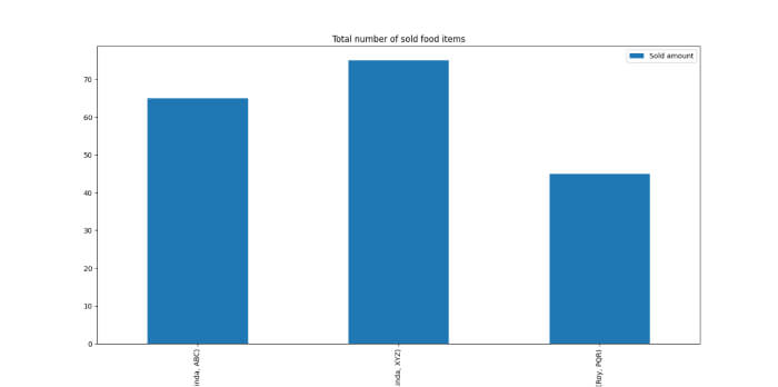
We can visualize our pivot table as a bar chart, pie chart, or other type. To visualize the pivot table, we can use the plot function, which the matplotlib library provides.
import matplotlib.pyplot as plt

sold_amount = df.pivot_table(index=['Account manager', 'Restaurant name'], values='Sold amount', aggfunc=sum)

sold_amount.plot.bar(figsize=(8,8), title='Total number of sold food items')

plt.show()
Here, we are visualizing our pivot table as a bar chart as follows.

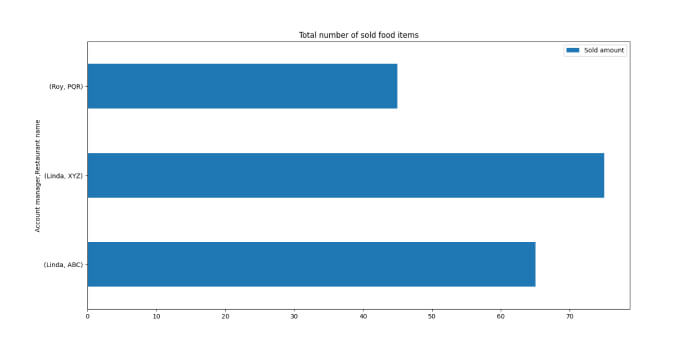
We can make it a horizontal bar chart by changing the ‘bar’ keyword to ‘barh.’
sold_amount.plot.barh(figsize=(8,8), title='Total number of sold food items')

plt.show()
We will get our horizontal bar chart, as shown below.

Conclusion
Today, we learned one of the most significant features provided by the Python Pandas library: Pivot tables. As discussed, pivot tables are very beneficial when analyzing and reporting data sets. We saw what data pivoting and pivot() function do and then had a brief introduction to pivot tables in Pandas. We learned the syntax of the pivot_table() function, how to create one, pivot table aggregations and different aggregation functions, visualize pivot tables, and many more valuable concepts. By learning these concepts, we can make our data analysis processes much easier and get accuracy-improved analysis reports.


